Kaggle Titanic (Top 6%)
1. Introduction
This notebook is a take on the legendary Kaggle Titanic Machine Learning competition.
RMS Titanic was a British passenger liner that sank in the North Atlantic Ocean in 1912 after striking an iceberg during her maiden voyage from Southampton to New York City. Of the estimated 2,224 passengers and crew aboard, more than 1,500 died, making the sinking one of modern history’s deadliest peacetime commercial marine disasters. (Wikipedia)
In this Kaggle challenge, the goal is to build a predictive model that answers the question: “what sorts of people were more likely to survive?” using passenger data (ie name, age, gender, socio-economic class, etc).

2. Imports
2.1. Import Librairies and Tools
Let’s import the packages needed to perform this analysis.
import pandas as pd
print("Pandas version: {}".format(pd.__version__))

import numpy as np
print("Numpy version: {}".format(np.__version__))

import matplotlib
import matplotlib.pyplot as plt
fs = (16,6) # Figure size
print("Matplotlib version: {}".format(matplotlib.__version__))

import scipy as sp
print("Scipy version: {}".format(sp.__version__))

import sklearn
from sklearn.linear_model import LogisticRegression, PassiveAggressiveClassifier, RidgeClassifier, SGDClassifier, Perceptron
from sklearn.tree import DecisionTreeClassifier, DecisionTreeRegressor
from sklearn.model_selection import cross_val_score,GridSearchCV, StratifiedKFold, train_test_split
from sklearn.naive_bayes import GaussianNB, BernoulliNB
from sklearn.tree import DecisionTreeClassifier
from sklearn.ensemble import VotingClassifier, RandomForestClassifier, GradientBoostingClassifier, BaggingClassifier, AdaBoostClassifier, ExtraTreesClassifier
from sklearn.svm import SVC, NuSVC, LinearSVC
from sklearn.preprocessing import StandardScaler
from sklearn.discriminant_analysis import LinearDiscriminantAnalysis, QuadraticDiscriminantAnalysis
from sklearn.neighbors import KNeighborsClassifier
from sklearn.gaussian_process import GaussianProcessClassifier
from sklearn.neural_network import MLPClassifier
print("Sklearn version: {}".format(sklearn.__version__))

import xgboost
from xgboost import XGBClassifier
print("Xgboost version: {}".format(xgboost.__version__))

import seaborn as sns
print("Seaborn version: {}".format(sns.__version__))

import IPython
from IPython.display import display
print("IPython version: {}".format(IPython.__version__))

%matplotlib inline

# Do not show warnings (used when the notebook is completed)
import warnings
# warnings.filterwarnings('ignore') !!!
Pandas version: 0.25.3
Numpy version: 1.18.1
Matplotlib version: 3.1.2
Scipy version: 1.3.2
Sklearn version: 0.22.1
Xgboost version: 0.90
Seaborn version: 0.9.0
IPython version: 7.11.1
2.2. Import Data
Data is provided on the Kaggle website (https://www.kaggle.com/c/titanic/data), downloaded locally and imported below. It consists of one train set (with the gound-truth of the survival of the passengers) and the test set (without the survival of passengers).
train0 = pd.read_csv('train.csv')
test0 = pd.read_csv('test.csv')

train = train0.copy() # train will be modified throughout this notebook
test = test0.copy() # test will be modified throughout this notebook
3. Data Overview
3.1. Log of data set modifications
The following lists the modifications made to the train, test and/ or ds set (train+test), and the Section where it was made.
- Overview and pre-cleaning: dropped “PassengerId” columns from all sets.
- Fare: filled one missing “Fare” value in the test set.
- Embarkment: filled two missing “Embarkment” values in the train set.
- Age Filling: Filled missing “Age” values from train and test set.
- Statistical Analysis: replaced the “Sex” data with 0 or 1 in all sets.
- Age Groups: Added “Age” groups to all sets.
- Class Groups: Added “Pclass” groups to all sets.
3.2. Fields
The following fields are present in the data (according to Kaggle):
Survived Survival, 0 = No, 1 = Yes
Pclass Ticket class, 1 = 1st, 2 = 2nd, 3 = 3rd
Sex Gender
Age Age in years Age is fractional if less than 1. If the age is estimated, is it in the form of xx.5
SibSp # of siblings / spouses aboard the Titanic
Parch # of parents / children aboard the Titanic
Ticket Ticket number
Fare Passenger fare
Cabin Cabin number
Embarked Port of Embarkation, C = Cherbourg, Q = Queenstown, S = Southampton.
3.3. Overview and pre-cleaning
Let’s take a look at the data and do basic cleaning to make handling it easier.
print('The train dataset contains {} entries. Preview:'.format(str(train.shape[0])))
display(train.head())
print('The test dataset contains {} entries. Preview:'.format(str(test.shape[0])))
display(test.head())
The train dataset contains 891 entries. Preview:
| PassengerId | Survived | Pclass | Name | Sex | Age | SibSp | Parch | Ticket | Fare | Cabin | Embarked | |
|---|---|---|---|---|---|---|---|---|---|---|---|---|
| 0 | 1 | 0 | 3 | Braund, Mr. Owen Harris | male | 22.0 | 1 | 0 | A/5 21171 | 7.2500 | NaN | S |
| 1 | 2 | 1 | 1 | Cumings, Mrs. John Bradley (Florence Briggs Th... | female | 38.0 | 1 | 0 | PC 17599 | 71.2833 | C85 | C |
| 2 | 3 | 1 | 3 | Heikkinen, Miss. Laina | female | 26.0 | 0 | 0 | STON/O2. 3101282 | 7.9250 | NaN | S |
| 3 | 4 | 1 | 1 | Futrelle, Mrs. Jacques Heath (Lily May Peel) | female | 35.0 | 1 | 0 | 113803 | 53.1000 | C123 | S |
| 4 | 5 | 0 | 3 | Allen, Mr. William Henry | male | 35.0 | 0 | 0 | 373450 | 8.0500 | NaN | S |
The test dataset contains 418 entries. Preview:
| PassengerId | Pclass | Name | Sex | Age | SibSp | Parch | Ticket | Fare | Cabin | Embarked | |
|---|---|---|---|---|---|---|---|---|---|---|---|
| 0 | 892 | 3 | Kelly, Mr. James | male | 34.5 | 0 | 0 | 330911 | 7.8292 | NaN | Q |
| 1 | 893 | 3 | Wilkes, Mrs. James (Ellen Needs) | female | 47.0 | 1 | 0 | 363272 | 7.0000 | NaN | S |
| 2 | 894 | 2 | Myles, Mr. Thomas Francis | male | 62.0 | 0 | 0 | 240276 | 9.6875 | NaN | Q |
| 3 | 895 | 3 | Wirz, Mr. Albert | male | 27.0 | 0 | 0 | 315154 | 8.6625 | NaN | S |
| 4 | 896 | 3 | Hirvonen, Mrs. Alexander (Helga E Lindqvist) | female | 22.0 | 1 | 1 | 3101298 | 12.2875 | NaN | S |
The PassengerId field does not bring any information (members of the same family are not listed sequentially). This field is deleted from the train and test dataset.
# Delete PassengerId field
train.drop('PassengerId', axis=1, inplace=True)
test.drop('PassengerId', axis=1, inplace=True)
Let’s create a unique DataFram ‘ds’ that combines the train and test set.
# Combine train and test sets into ds ('dataset'), dropping the 'Survived' column for the train set.
ds = pd.concat([train.drop('Survived', axis=1), test], axis=0)
print("Preview of combined dataset 'ds':")
display(ds.head())
print('...')
ds.tail()
Preview of combined dataset 'ds':
| Pclass | Name | Sex | Age | SibSp | Parch | Ticket | Fare | Cabin | Embarked | |
|---|---|---|---|---|---|---|---|---|---|---|
| 0 | 3 | Braund, Mr. Owen Harris | male | 22.0 | 1 | 0 | A/5 21171 | 7.2500 | NaN | S |
| 1 | 1 | Cumings, Mrs. John Bradley (Florence Briggs Th... | female | 38.0 | 1 | 0 | PC 17599 | 71.2833 | C85 | C |
| 2 | 3 | Heikkinen, Miss. Laina | female | 26.0 | 0 | 0 | STON/O2. 3101282 | 7.9250 | NaN | S |
| 3 | 1 | Futrelle, Mrs. Jacques Heath (Lily May Peel) | female | 35.0 | 1 | 0 | 113803 | 53.1000 | C123 | S |
| 4 | 3 | Allen, Mr. William Henry | male | 35.0 | 0 | 0 | 373450 | 8.0500 | NaN | S |
...
| Pclass | Name | Sex | Age | SibSp | Parch | Ticket | Fare | Cabin | Embarked | |
|---|---|---|---|---|---|---|---|---|---|---|
| 413 | 3 | Spector, Mr. Woolf | male | NaN | 0 | 0 | A.5. 3236 | 8.0500 | NaN | S |
| 414 | 1 | Oliva y Ocana, Dona. Fermina | female | 39.0 | 0 | 0 | PC 17758 | 108.9000 | C105 | C |
| 415 | 3 | Saether, Mr. Simon Sivertsen | male | 38.5 | 0 | 0 | SOTON/O.Q. 3101262 | 7.2500 | NaN | S |
| 416 | 3 | Ware, Mr. Frederick | male | NaN | 0 | 0 | 359309 | 8.0500 | NaN | S |
| 417 | 3 | Peter, Master. Michael J | male | NaN | 1 | 1 | 2668 | 22.3583 | NaN | C |
3.4. Missing data
# Inspect and look for missing data in the training set
temp = train.isna().sum(axis=0)
print('Training set missing data:')
print(temp[temp>0])
Training set missing data:
Age         177
Cabin       687
Embarked      2
dtype: int64
# Inspect and look for missing data in the training set
temp = test.isna().sum(axis=0)
print('Test set missing data:')
print(temp[temp>0])
Test set missing data:
Age       86
Fare       1
Cabin    327
dtype: int64
3.4.1. Missing Age Data
Age data is missing from a substantial number of data entries, about 20% for the train set. Filling the missing values with the average or median would be too simplistic, given that age is most likely an important parameter for survival rate. A more advanced evaluation will be performed later in this notebook.
3.4.2. Missing Cabin Data
# Correlation between cabin and class
cabin_temp = ds.dropna(axis=0, subset=['Cabin'])
cabin_temp.head(5)
| Pclass | Name | Sex | Age | SibSp | Parch | Ticket | Fare | Cabin | Embarked | |
|---|---|---|---|---|---|---|---|---|---|---|
| 1 | 1 | Cumings, Mrs. John Bradley (Florence Briggs Th... | female | 38.0 | 1 | 0 | PC 17599 | 71.2833 | C85 | C |
| 3 | 1 | Futrelle, Mrs. Jacques Heath (Lily May Peel) | female | 35.0 | 1 | 0 | 113803 | 53.1000 | C123 | S |
| 6 | 1 | McCarthy, Mr. Timothy J | male | 54.0 | 0 | 0 | 17463 | 51.8625 | E46 | S |
| 10 | 3 | Sandstrom, Miss. Marguerite Rut | female | 4.0 | 1 | 1 | PP 9549 | 16.7000 | G6 | S |
| 11 | 1 | Bonnell, Miss. Elizabeth | female | 58.0 | 0 | 0 | 113783 | 26.5500 | C103 | S |
Let’s extract the cabin deck from the Cabin field and create a new field ‘Deck’.
# Extract the letter from the cabin
cabin_temp['Deck']=cabin_temp['Cabin'].apply(lambda x: x[0])
cabin_temp.head(5)
C:\ProgramData\Anaconda3\lib\site-packages\ipykernel_launcher.py:2: SettingWithCopyWarning:
A value is trying to be set on a copy of a slice from a DataFrame.
Try using .loc[row_indexer,col_indexer] = value instead

See the caveats in the documentation: http://pandas.pydata.org/pandas-docs/stable/user_guide/indexing.html#returning-a-view-versus-a-copy
| Pclass | Name | Sex | Age | SibSp | Parch | Ticket | Fare | Cabin | Embarked | Deck | |
|---|---|---|---|---|---|---|---|---|---|---|---|
| 1 | 1 | Cumings, Mrs. John Bradley (Florence Briggs Th... | female | 38.0 | 1 | 0 | PC 17599 | 71.2833 | C85 | C | C |
| 3 | 1 | Futrelle, Mrs. Jacques Heath (Lily May Peel) | female | 35.0 | 1 | 0 | 113803 | 53.1000 | C123 | S | C |
| 6 | 1 | McCarthy, Mr. Timothy J | male | 54.0 | 0 | 0 | 17463 | 51.8625 | E46 | S | E |
| 10 | 3 | Sandstrom, Miss. Marguerite Rut | female | 4.0 | 1 | 1 | PP 9549 | 16.7000 | G6 | S | G |
| 11 | 1 | Bonnell, Miss. Elizabeth | female | 58.0 | 0 | 0 | 113783 | 26.5500 | C103 | S | C |
# Show Cabin Letter Distribution with Pclass
cabin_temp[['Pclass', 'Deck', 'Fare']].groupby(['Pclass', 'Deck']).mean()
| Fare | ||
|---|---|---|
| Pclass | Deck | |
| 1 | A | 41.244314 |
| B | 122.383078 | |
| C | 107.926598 | |
| D | 58.919065 | |
| E | 63.464706 | |
| T | 35.500000 | |
| 2 | D | 13.595833 |
| E | 11.587500 | |
| F | 23.423077 | |
| 3 | E | 11.000000 |
| F | 9.395838 | |
| G | 14.205000 |
From the above results, we see that 1st class has cabins A, B, C, D and T exclusively, but they share cabin D with 2nd class and cabin E with 2nd class and 3rd class. Cabin F is shared with 2nd and 3rd class and Cabin G is only for 3rd class passengers.
For a better understanding, let’s see how the cabin influence the survival rate.
temp = train.dropna(axis=0, subset=['Cabin'])
temp['Deck']=temp['Cabin'].apply(lambda x: x[0])
temp[['Pclass', 'Survived', 'Deck']].groupby(['Pclass', 'Deck']).mean()
C:\ProgramData\Anaconda3\lib\site-packages\ipykernel_launcher.py:2: SettingWithCopyWarning:
A value is trying to be set on a copy of a slice from a DataFrame.
Try using .loc[row_indexer,col_indexer] = value instead

See the caveats in the documentation: http://pandas.pydata.org/pandas-docs/stable/user_guide/indexing.html#returning-a-view-versus-a-copy
| Survived | ||
|---|---|---|
| Pclass | Deck | |
| 1 | A | 0.466667 |
| B | 0.744681 | |
| C | 0.593220 | |
| D | 0.758621 | |
| E | 0.720000 | |
| T | 0.000000 | |
| 2 | D | 0.750000 |
| E | 0.750000 | |
| F | 0.875000 | |
| 3 | E | 1.000000 |
| F | 0.200000 | |
| G | 0.500000 |
temp[['Pclass', 'Survived', 'Deck']].groupby(['Pclass', 'Deck']).count()
| Survived | ||
|---|---|---|
| Pclass | Deck | |
| 1 | A | 15 |
| B | 47 | |
| C | 59 | |
| D | 29 | |
| E | 25 | |
| T | 1 | |
| 2 | D | 4 |
| E | 4 | |
| F | 8 | |
| 3 | E | 3 |
| F | 5 | |
| G | 4 |
It seems like there are enough data in the 1st class passengers to have a correlation between the fare and the cabin. Let’s display a bar plot to see if it would be feasible to tie the fare back to the deck, knowing the class.
sns.set(rc={'figure.figsize':(12,8)})
sns.boxplot(x=temp['Deck'], y=temp['Fare'], hue=temp['Pclass'])
plt.ylim(0,300)
(0, 300)

It seems difficult to predict accurately the Deck based on the fare and the class. The existing decks will be used by algorithm able to use incomplete features.
3.4.3. Missing Embarkment Data
train[train['Embarked'].isna()]
| Survived | Pclass | Name | Sex | Age | SibSp | Parch | Ticket | Fare | Cabin | Embarked | |
|---|---|---|---|---|---|---|---|---|---|---|---|
| 61 | 1 | 1 | Icard, Miss. Amelie | female | 38.0 | 0 | 0 | 113572 | 80.0 | B28 | NaN |
| 829 | 1 | 1 | Stone, Mrs. George Nelson (Martha Evelyn) | female | 62.0 | 0 | 0 | 113572 | 80.0 | B28 | NaN |
Let’s display the correlation between the embrarkment, the class and the fare for the whole set (train+test).
sns.boxplot(x=ds['Embarked'], y=ds['Fare'], hue=ds['Pclass'])
plt.ylim(0,200);
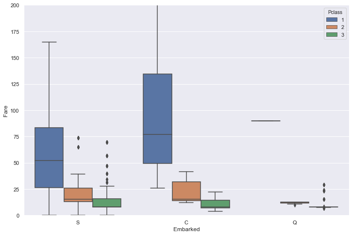
Embarkment C seems a reasonable assumption for these two women in 1st class who paid $$80.
# Fill the missing information
train.loc[train['Embarked'].isna(),'Embarked']=['C']
4. Data Visualization and Feature Exploration
Let’s vizualize the survival rate with respect to criteria that appear essential in survival, namely the class, the gender, the age and the size of the family.
4.1. Class
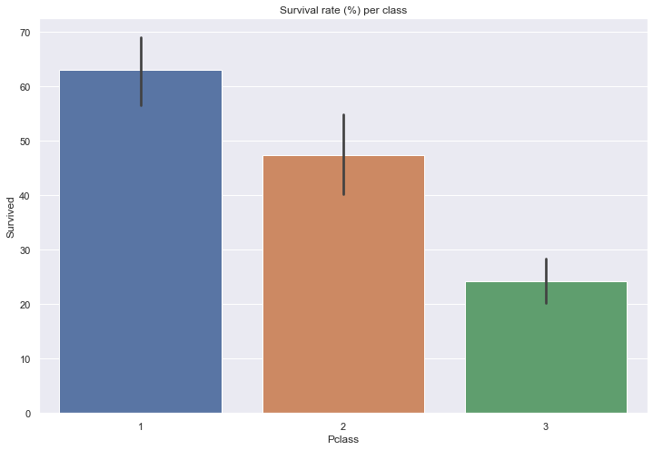
Let’s display the survival rate as a function of the passenger class.
print(train[['Pclass', 'Survived']].groupby(['Pclass']).mean().round(3)*100)
sns.barplot(x=train['Pclass'], y=train['Survived']*100)
plt.title('Survival rate (%) per class')
        Survived
Pclass
1           63.0
2           47.3
3           24.2


Text(0.5, 1.0, 'Survival rate (%) per class')
Let’s verify the fare is correlated to the class.
print(train[['Fare', 'Pclass']].groupby(['Pclass']).mean().round(1))
sns.barplot(x=train['Pclass'], y=train['Fare'])
plt.title('Survival rate (%) per class')
        Fare
Pclass
1       84.2
2       20.7
3       13.7


Text(0.5, 1.0, 'Survival rate (%) per class')

Let’s look at the importance of the fare variation within a class.
sns.boxplot(train['Pclass'], train['Fare'], hue=train['Survived'])
plt.ylim(0,200); # Extreme fares removed for clarity

There is a correlation between the fare and the survival rate within a class, especially for the upper classes.
4.2. Gender
Let’s look at the importance of gender over the survival rate.
sns.barplot(train['Sex'], train['Survived'], hue=train['Pclass'])
plt.title("Impact of gender (and class) on survival rate")
Text(0.5, 1.0, 'Impact of gender (and class) on survival rate')
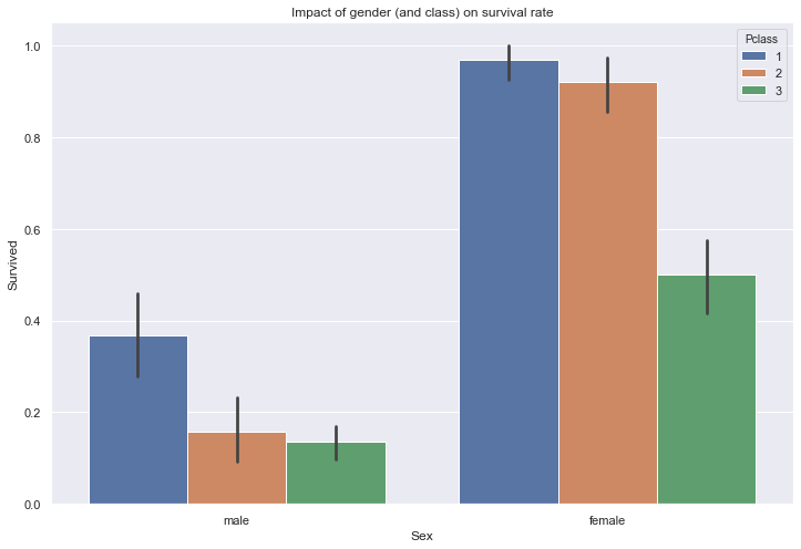
As expected, women have a significantly higher survival rate than men across all passenger classes.
4.3. Age
4.3.1. Age Visualization
Let’s look at the importance of age for the survival rate.
sns.kdeplot(train.loc[train['Survived']==1,'Age'], label="Survived", shade=True, color='green')
sns.kdeplot(train.loc[train['Survived']==0,'Age'], label="Did not survive", shade=True, color='gray')
sns.kdeplot(train['Age'], label="All passengers", shade=False, color='black')
plt.xticks(np.arange(0, 80, 2.0))
plt.title('Survival rate as a function of age')
plt.xlabel('Age'); plt.ylabel('Frequency');
plt.gcf().set_size_inches(20,12)
C:\ProgramData\Anaconda3\lib\site-packages\statsmodels\nonparametric\kde.py:447: RuntimeWarning: invalid value encountered in greater
  X = X[np.logical_and(X > clip[0], X < clip[1])] # won't work for two columns.
C:\ProgramData\Anaconda3\lib\site-packages\statsmodels\nonparametric\kde.py:447: RuntimeWarning: invalid value encountered in less
  X = X[np.logical_and(X > clip[0], X < clip[1])] # won't work for two columns.

From the above plot, it appears that young adults younger than 12 have a higher survival rate, especially infants and toddlers (0-3 year old). On the other hand. Teenagers and young adults (13-30 year old) have a low survival rate. After 58 year old, the survival rate decreases with age.
sns.kdeplot(train.loc[(train['Survived']==1) & (train['Sex']=='female'),'Age'], label="Survived female", shade=True, color='green')
# sns.kdeplot(train.loc[(train['Survived']==1) & (train['Sex']=='male'),'Age'], label="Survived male", shade=True, color='gray')
sns.kdeplot(train.loc[train['Sex']=='female','Age'], label="All female passengers", shade=False, color='black')
plt.xticks(np.arange(0, 80, 2.0))
plt.title('Survival rate for women as a function of age')
plt.xlabel('Age'); plt.ylabel('Frequency');
plt.gcf().set_size_inches(20,12)
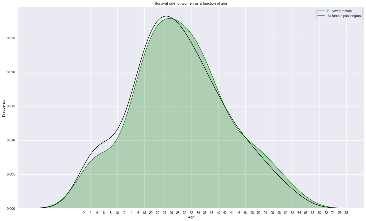
Surival of women is little influenced by age. Younger women tend to have a slightly lower survival rate.
sns.kdeplot(train.loc[(train['Survived']==1) & (train['Sex']=='male'),'Age'], label="Survived male", shade=True, color='green')
# sns.kdeplot(train.loc[(train['Survived']==1) & (train['Sex']=='male'),'Age'], label="Survived male", shade=True, color='gray')
sns.kdeplot(train.loc[train['Sex']=='male','Age'], label="All male passengers", shade=False, color='black')
plt.xticks(np.arange(0, 80, 2.0))
plt.title('Survival rate for men as a function of age')
plt.xlabel('Age'); plt.ylabel('Frequency');
plt.gcf().set_size_inches(20,12)
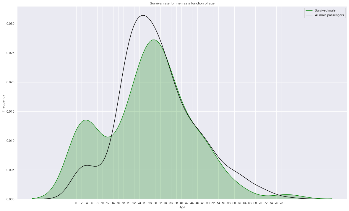
Survival of men is significantly influenced by their age. While young kids have a much higher survival rate, young men (14-34 years old) have a low surival rate (influenced by class) and men older than 50 have a lower survival rate (influenced by age).
4.4. Family members
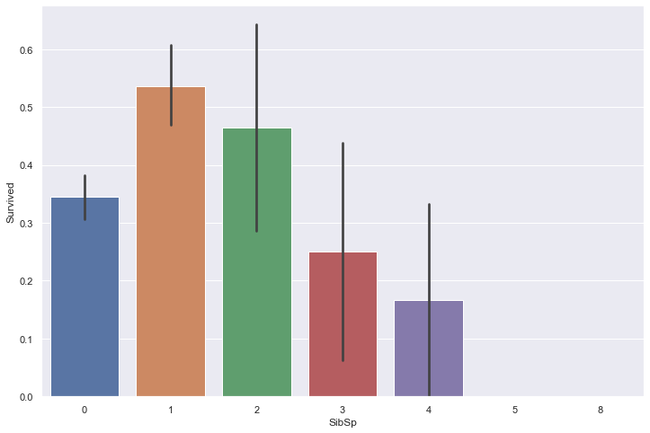
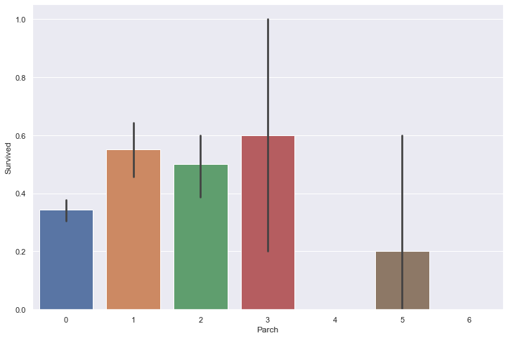
The Sibsp field is the number of siblings (brother, sister, stepbrother, stepsister) and spouses (husband or wife, mistresses and fiancés were ignored) aboard the Titanic, while the Parch field is the number of parents (mother, father) and children (daughter, son, stepdaughter, stepson) aboard the Titanic. Some children travelled only with a nanny, therefore parch=0 for them.
Let’s plot the survival rate as a function of these two fields.
sns.barplot(train['SibSp'], train['Survived'])
<matplotlib.axes._subplots.AxesSubplot at 0x234b9f81508>
sns.barplot(train['Parch'], train['Survived'])
<matplotlib.axes._subplots.AxesSubplot at 0x234ba59da08>
temp = (train.loc[:,['Survived','SibSp', 'Parch']].groupby(['SibSp', 'Parch']).mean())
temp = pd.pivot_table(temp,index='SibSp',columns='Parch')
sns.heatmap(temp,xticklabels=range(7))
plt.xlabel('Parch')
plt.title('Survival heat map as a function of SibSp and Parch')
Text(0.5, 1, 'Survival heat map as a function of SibSp and Parch')
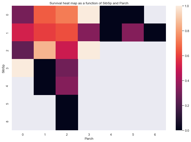
It appears that small sized families have a higher survival rate than single people and large families.
4.5. Embarkment
sns.barplot(train['Embarked'], train['Survived'])
<matplotlib.axes._subplots.AxesSubplot at 0x234ba9d3288>

sns.barplot(train['Embarked'], train['Survived'], hue=train['Pclass'])
<matplotlib.axes._subplots.AxesSubplot at 0x234ba627e08>
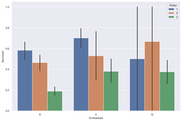
The port of embrakation seems to play a role at first sight, but by breaking down each port into passenger class, it seems that the variation of survival rate comes from a different distribution of passenger rather than the port itself.
4.6. Title (see age, delete this section?)
4.7. Reamining missing data
# Inspect and look for missing data in the training set
temp = train.isna().sum(axis=0)
print('Training set missing data:')
temp[temp>0] # good practice ????? !!!
Training set missing data:


Age      177
Cabin    687
dtype: int64
A lot of the data is missing for the cabin field. For now, that field is ignored.
ds.drop(['Cabin'], axis=1, inplace=True)
train.drop(['Cabin'], axis=1, inplace=True)
test.drop(['Cabin'], axis=1, inplace=True);
5. Statistical Analysis
According to the previous section, the following fields are important in determining the surival rate: Age, Pclass, Sex, Fare, SibSp, Parch. All these fields are numerical except the Sex category. Let’s turn this field into a numerical category using 0 for women and 1 for men.
train['Sex']=train['Sex'].apply(lambda s: 0 if s=='female' else 1)
test['Sex']=test['Sex'].apply(lambda s: 0 if s=='female' else 1)
ds['Sex']=ds['Sex'].apply(lambda s: 0 if s=='female' else 1)
train.describe()
| Survived | Pclass | Sex | Age | SibSp | Parch | Fare | |
|---|---|---|---|---|---|---|---|
| count | 891.000000 | 891.000000 | 891.000000 | 714.000000 | 891.000000 | 891.000000 | 891.000000 |
| mean | 0.383838 | 2.308642 | 0.647587 | 29.699118 | 0.523008 | 0.381594 | 32.204208 |
| std | 0.486592 | 0.836071 | 0.477990 | 14.526497 | 1.102743 | 0.806057 | 49.693429 |
| min | 0.000000 | 1.000000 | 0.000000 | 0.420000 | 0.000000 | 0.000000 | 0.000000 |
| 25% | 0.000000 | 2.000000 | 0.000000 | 20.125000 | 0.000000 | 0.000000 | 7.910400 |
| 50% | 0.000000 | 3.000000 | 1.000000 | 28.000000 | 0.000000 | 0.000000 | 14.454200 |
| 75% | 1.000000 | 3.000000 | 1.000000 | 38.000000 | 1.000000 | 0.000000 | 31.000000 |
| max | 1.000000 | 3.000000 | 1.000000 | 80.000000 | 8.000000 | 6.000000 | 512.329200 |
Let’s plot a survival rate correlation heatmap.
train.corr()
| Survived | Pclass | Sex | Age | SibSp | Parch | Fare | |
|---|---|---|---|---|---|---|---|
| Survived | 1.000000 | -0.338481 | -0.543351 | -0.077221 | -0.035322 | 0.081629 | 0.257307 |
| Pclass | -0.338481 | 1.000000 | 0.131900 | -0.369226 | 0.083081 | 0.018443 | -0.549500 |
| Sex | -0.543351 | 0.131900 | 1.000000 | 0.093254 | -0.114631 | -0.245489 | -0.182333 |
| Age | -0.077221 | -0.369226 | 0.093254 | 1.000000 | -0.308247 | -0.189119 | 0.096067 |
| SibSp | -0.035322 | 0.083081 | -0.114631 | -0.308247 | 1.000000 | 0.414838 | 0.159651 |
| Parch | 0.081629 | 0.018443 | -0.245489 | -0.189119 | 0.414838 | 1.000000 | 0.216225 |
| Fare | 0.257307 | -0.549500 | -0.182333 | 0.096067 | 0.159651 | 0.216225 | 1.000000 |
n_colors = 256 # Number of colors in the legend bar
color_min, color_max = [-1, 1] # Range of values that will be mapped to the palette, i.e. min and max possible correlation

heatmap_columns = ['Survived', 'Age', 'Pclass', 'Sex', 'Fare', 'SibSp', 'Parch']

def heatmap(x, y, size, color, palette):
#     fig, ax = plt.subplots()
    plot_grid = plt.GridSpec(1, 15, hspace=0.2, wspace=0.1) # Setup a 1x15 grid
    ax = plt.subplot(plot_grid[:,:-1]) # Use the leftmost 14 columns of the grid for the main plot
    # Mapping from column names to integer coordinates
    x_labels = heatmap_columns[:-1:]
    y_labels = heatmap_columns[::-1][:-1]
    x_to_num = {p[1]:p[0] for p in enumerate(x_labels)}
    y_to_num = {p[1]:p[0] for p in enumerate(y_labels)}
    size_scale = 3000

    ax.scatter(x=x.map(x_to_num), y=y.map(y_to_num),s=size*size_scale, c=color, cmap=palette, marker='s')

    plt.title('Correlation between the main features.')
    ax.set_xticks([x_to_num[v] for v in x_labels])
    ax.set_xticklabels(x_labels, rotation=45, horizontalalignment='right')
    ax.set_yticks([y_to_num[v] for v in y_labels])
    ax.set_yticklabels(y_labels)
    ax.grid(False, 'major')
    ax.grid(True, 'minor')
    ax.set_xticks([t + 0.5 for t in ax.get_xticks()], minor=True)
    ax.set_yticks([t + 0.5 for t in ax.get_yticks()], minor=True)
    ax.set_xlim([-0.5, max([v for v in x_to_num.values()]) + 0.5])
    ax.set_ylim([-0.5, max([v for v in y_to_num.values()]) + 0.5])

#     # Add color legend on the right side of the plot
    ax = plt.subplot(plot_grid[:,-1]) # Use the rightmost column of the plot

    col_x = [0]*50 # Fixed x coordinate for the bars
    bar_y=np.linspace(color_min, color_max, n_colors) # y coordinates for each of the n_colors bars
    bar_height = bar_y[1] - bar_y[0]

    ax.barh(y=bar_y,
        width=5, # Make bars 5 units wide
        left=0, # Make bars start at 0
        height=bar_height,
        color=palette(bar_y+0.5),
        linewidth=0)

    ax.set_xticklabels([])
    ax.yaxis.tick_right()
    ax.set_ylim(-1,1)

corr = train[heatmap_columns].corr()
corr = corr.mask(np.tril(np.ones(corr.shape)).astype(np.bool)) # Removes the upper triangle diagonal
corr = pd.melt(corr.reset_index(), id_vars='index') # Unpivot the dataframe, so we can get pair of arrays for x and y
corr.columns = ['x', 'y', 'value']
# print(corr)
heatmap(
    x=corr['x'],
    y=corr['y'],
    size=corr['value'].abs(),
    color = corr['value'],
    palette=plt.cm.bwr
)

plt.gcf().set_size_inches(10,10)
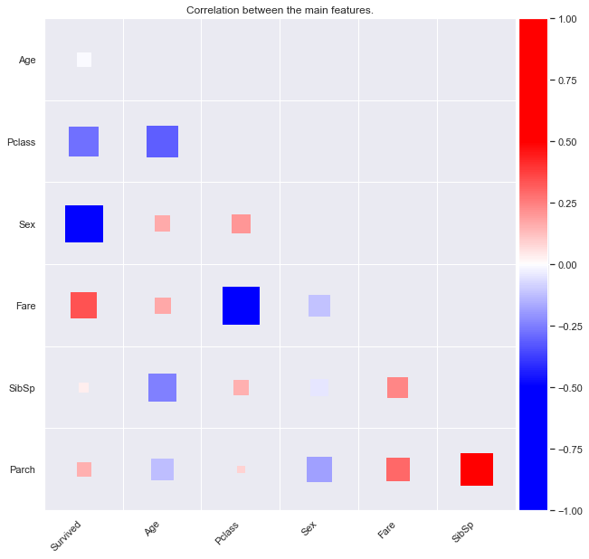
In the above plot, the correlation between feature is shown with both color and size for an easy understanding. The size is proportional to the correlation, positive or negative.
6. Data Filling
6.1. Age Filling
Title may have an impact on the survival rate. Let’s extract the title from the Name field.
# Extract the title from the names
ds['Title']=ds['Name'].str.extract(r'([A-Za-z]+)\.',expand=False)
train['Title']=train['Name'].str.extract(r'([A-Za-z]+)\.',expand=False)
test['Title']=test['Name'].str.extract(r'([A-Za-z]+)\.',expand=False)
ds['Title'].value_counts()
Mr          757
Miss        260
Mrs         197
Master       61
Dr            8
Rev           8
Col           4
Major         2
Ms            2
Mlle          2
Lady          1
Sir           1
Don           1
Countess      1
Capt          1
Mme           1
Dona          1
Jonkheer      1
Name: Title, dtype: int64
ds.groupby(['Title'])['Age'].agg(['mean','std']).sort_values(['mean'])
| mean | std | |
|---|---|---|
| Title | ||
| Master | 5.482642 | 4.161554 |
| Miss | 21.774238 | 12.249077 |
| Mlle | 24.000000 | 0.000000 |
| Mme | 24.000000 | NaN |
| Ms | 28.000000 | NaN |
| Mr | 32.252151 | 12.422089 |
| Countess | 33.000000 | NaN |
| Mrs | 36.994118 | 12.901767 |
| Jonkheer | 38.000000 | NaN |
| Dona | 39.000000 | NaN |
| Don | 40.000000 | NaN |
| Rev | 41.250000 | 12.020815 |
| Dr | 43.571429 | 11.731115 |
| Lady | 48.000000 | NaN |
| Major | 48.500000 | 4.949747 |
| Sir | 49.000000 | NaN |
| Col | 54.000000 | 5.477226 |
| Capt | 70.000000 | NaN |
It’s interesting to notice that “Master” is a title for young boys! Based on the mean and standard deviation, the title seems to be a reasonable estimate for the age.
def fill_age(df):
    titles_map = ds.loc[:,['Title','Age']].groupby(['Title']).mean().sort_values(['Age'])
    age_from_titles = df.loc[:,'Title'].apply(lambda x: titles_map.loc[x].values[0])
    df['Age']=df['Age'].fillna(age_from_titles)
    return df
fill_age(train)
fill_age(test)
fill_age(ds)
| Pclass | Name | Sex | Age | SibSp | Parch | Ticket | Fare | Embarked | Title | |
|---|---|---|---|---|---|---|---|---|---|---|
| 0 | 3 | Braund, Mr. Owen Harris | 1 | 22.000000 | 1 | 0 | A/5 21171 | 7.2500 | S | Mr |
| 1 | 1 | Cumings, Mrs. John Bradley (Florence Briggs Th... | 0 | 38.000000 | 1 | 0 | PC 17599 | 71.2833 | C | Mrs |
| 2 | 3 | Heikkinen, Miss. Laina | 0 | 26.000000 | 0 | 0 | STON/O2. 3101282 | 7.9250 | S | Miss |
| 3 | 1 | Futrelle, Mrs. Jacques Heath (Lily May Peel) | 0 | 35.000000 | 1 | 0 | 113803 | 53.1000 | S | Mrs |
| 4 | 3 | Allen, Mr. William Henry | 1 | 35.000000 | 0 | 0 | 373450 | 8.0500 | S | Mr |
| ... | ... | ... | ... | ... | ... | ... | ... | ... | ... | ... |
| 413 | 3 | Spector, Mr. Woolf | 1 | 32.252151 | 0 | 0 | A.5. 3236 | 8.0500 | S | Mr |
| 414 | 1 | Oliva y Ocana, Dona. Fermina | 0 | 39.000000 | 0 | 0 | PC 17758 | 108.9000 | C | Dona |
| 415 | 3 | Saether, Mr. Simon Sivertsen | 1 | 38.500000 | 0 | 0 | SOTON/O.Q. 3101262 | 7.2500 | S | Mr |
| 416 | 3 | Ware, Mr. Frederick | 1 | 32.252151 | 0 | 0 | 359309 | 8.0500 | S | Mr |
| 417 | 3 | Peter, Master. Michael J | 1 | 5.482642 | 1 | 1 | 2668 | 22.3583 | C | Master |
1309 rows × 10 columns
6.2. Fare Filling
Let’s impact the one missing ‘fare’ from the test set.
test.loc[test['Fare'].isna(),:]
| Pclass | Name | Sex | Age | SibSp | Parch | Ticket | Fare | Embarked | Title | |
|---|---|---|---|---|---|---|---|---|---|---|
| 152 | 3 | Storey, Mr. Thomas | 1 | 60.5 | 0 | 0 | 3701 | NaN | S | Mr |
Let’s give this gentleman the mean fare from Misters in the 3r class.
temp_fare = ds.loc[:,['Pclass','Title','Fare']].groupby(['Pclass','Title']).mean().loc[3,:].loc['Mr'][0]
print('Average fare from Mister in the 3rd class: {} years.'.format(round(temp_fare,2)))
test.loc[test['Fare'].isna(),['Fare']] = temp_fare
Average fare from Mister in the 3rd class: 11.1 years.
7. Feature Engineering
7.1. Age Groups
Based on the results shown in previous sections, passengers are grouped into age groups as follows.
# def assign_age_group(age):
#     if age <= 12:
#         return "Child"
#     elif age <= 34:
#         return "Young adult"
#     elif age <= 50:
#         return "Adult"
#     else:
#         return "Senior"

def assign_age_group(age):
    if age <= 2:
        return "Toddler"
    elif age <= 12:
        return "Child"
    elif age <= 34:
        return "Young adult"
    elif age <= 50:
        return "Adult"
    else:
        return "Senior"
train['AgeGroup']=train['Age'].apply(lambda x: assign_age_group(x))
test['AgeGroup']=test['Age'].apply(lambda x: assign_age_group(x))
ds['AgeGroup']=ds['Age'].apply(lambda x: assign_age_group(x))
train = pd.concat((train, pd.get_dummies(train['AgeGroup'], prefix = 'AgeGroup', drop_first=True)), axis = 1)
test = pd.concat((test, pd.get_dummies(test['AgeGroup'], prefix = 'AgeGroup', drop_first=True)), axis = 1)
ds = pd.concat((ds, pd.get_dummies(ds['AgeGroup'], prefix = 'AgeGroup', drop_first=True)), axis = 1)
ds.head(3)
| Pclass | Name | Sex | Age | SibSp | Parch | Ticket | Fare | Embarked | Title | AgeGroup | AgeGroup_Child | AgeGroup_Senior | AgeGroup_Toddler | AgeGroup_Young adult | |
|---|---|---|---|---|---|---|---|---|---|---|---|---|---|---|---|
| 0 | 3 | Braund, Mr. Owen Harris | 1 | 22.0 | 1 | 0 | A/5 21171 | 7.2500 | S | Mr | Young adult | 0 | 0 | 0 | 1 |
| 1 | 1 | Cumings, Mrs. John Bradley (Florence Briggs Th... | 0 | 38.0 | 1 | 0 | PC 17599 | 71.2833 | C | Mrs | Adult | 0 | 0 | 0 | 0 |
| 2 | 3 | Heikkinen, Miss. Laina | 0 | 26.0 | 0 | 0 | STON/O2. 3101282 | 7.9250 | S | Miss | Young adult | 0 | 0 | 0 | 1 |
age_groups = ['AgeGroup_Child', 'AgeGroup_Senior', 'AgeGroup_Young adult']
7.2. Class Groups
As seen in an earlier Section, passenger class plays a key role in the survival of passengers, with the higher classes having a priviledge access to life boats. Passenger classes are here bined into three categories.
test['Pclass'].unique()
array([3, 2, 1], dtype=int64)
target = 'Pclass'
prefix = 'Pclass'

train = pd.concat((train, pd.get_dummies(train[target], prefix = prefix, drop_first=True)), axis = 1)
test = pd.concat((test, pd.get_dummies(test[target], prefix = prefix, drop_first=True)), axis = 1)
ds = pd.concat((ds, pd.get_dummies(ds[target], prefix = prefix, drop_first=True)), axis = 1)

class_groups = train.columns[-2:].to_list()
class_groups
['Pclass_2', 'Pclass_3']
test.head(1)
| Pclass | Name | Sex | Age | SibSp | Parch | Ticket | Fare | Embarked | Title | AgeGroup | AgeGroup_Child | AgeGroup_Senior | AgeGroup_Toddler | AgeGroup_Young adult | Pclass_2 | Pclass_3 | |
|---|---|---|---|---|---|---|---|---|---|---|---|---|---|---|---|---|---|
| 0 | 3 | Kelly, Mr. James | 1 | 34.5 | 0 | 0 | 330911 | 7.8292 | Q | Mr | Adult | 0 | 0 | 0 | 0 | 0 | 1 |
test['Pclass'].unique()
array([3, 2, 1], dtype=int64)
8. Model Inputs
ds.head(3)
| Pclass | Name | Sex | Age | SibSp | Parch | Ticket | Fare | Embarked | Title | AgeGroup | AgeGroup_Child | AgeGroup_Senior | AgeGroup_Toddler | AgeGroup_Young adult | Pclass_2 | Pclass_3 | |
|---|---|---|---|---|---|---|---|---|---|---|---|---|---|---|---|---|---|
| 0 | 3 | Braund, Mr. Owen Harris | 1 | 22.0 | 1 | 0 | A/5 21171 | 7.2500 | S | Mr | Young adult | 0 | 0 | 0 | 1 | 0 | 1 |
| 1 | 1 | Cumings, Mrs. John Bradley (Florence Briggs Th... | 0 | 38.0 | 1 | 0 | PC 17599 | 71.2833 | C | Mrs | Adult | 0 | 0 | 0 | 0 | 0 | 0 |
| 2 | 3 | Heikkinen, Miss. Laina | 0 | 26.0 | 0 | 0 | STON/O2. 3101282 | 7.9250 | S | Miss | Young adult | 0 | 0 | 0 | 1 | 0 | 1 |
selected_fields = ['Survived', 'Sex', 'SibSp', 'Parch', 'Fare']+age_groups+class_groups
print(selected_fields)
selected_fields_y = selected_fields.copy()
selected_fields_y.remove('Survived')
print(selected_fields_y)
['Survived', 'Sex', 'SibSp', 'Parch', 'Fare', 'AgeGroup_Child', 'AgeGroup_Senior', 'AgeGroup_Young adult', 'Pclass_2', 'Pclass_3']
['Sex', 'SibSp', 'Parch', 'Fare', 'AgeGroup_Child', 'AgeGroup_Senior', 'AgeGroup_Young adult', 'Pclass_2', 'Pclass_3']
X_train = train[selected_fields].drop(['Survived'],axis=1)
y_train = train['Survived']

X_test = test[selected_fields_y]
X_test.head(3)
| Sex | SibSp | Parch | Fare | AgeGroup_Child | AgeGroup_Senior | AgeGroup_Young adult | Pclass_2 | Pclass_3 | |
|---|---|---|---|---|---|---|---|---|---|
| 0 | 1 | 0 | 0 | 7.8292 | 0 | 0 | 0 | 0 | 1 |
| 1 | 0 | 1 | 0 | 7.0000 | 0 | 0 | 0 | 0 | 1 |
| 2 | 1 | 0 | 0 | 9.6875 | 0 | 1 | 0 | 1 | 0 |
X_train.head(3)
| Sex | SibSp | Parch | Fare | AgeGroup_Child | AgeGroup_Senior | AgeGroup_Young adult | Pclass_2 | Pclass_3 | |
|---|---|---|---|---|---|---|---|---|---|
| 0 | 1 | 1 | 0 | 7.2500 | 0 | 0 | 1 | 0 | 1 |
| 1 | 0 | 1 | 0 | 71.2833 | 0 | 0 | 0 | 0 | 0 |
| 2 | 0 | 0 | 0 | 7.9250 | 0 | 0 | 1 | 0 | 1 |
scaler = StandardScaler()
X_train = scaler.fit_transform(X_train)
X_test = scaler.transform(X_test)
9. Modeling
9.1. Classifiers Selection
# Cross validate model with Kfold stratified cross val
kfold = StratifiedKFold(n_splits=10)
random_state = 1986
n_jobs=-1 # The number of jobs to run in parallel for fit.
# classifiers
classifiers_list = [
    #Ensemble Methods
    AdaBoostClassifier(AdaBoostClassifier(DecisionTreeClassifier(random_state=random_state),random_state=random_state)),
    BaggingClassifier(random_state=random_state),
#     ExtraTreesClassifier(random_state=random_state),
    GradientBoostingClassifier(random_state=random_state),
    RandomForestClassifier(random_state=random_state),

    #Gaussian Processes
#     GaussianProcessClassifier(random_state=random_state),

    #GLM
    LogisticRegression(random_state=random_state),
#     PassiveAggressiveClassifier(random_state=random_state),
    RidgeClassifier(),
#     SGDClassifier(random_state=random_state),
#     Perceptron(random_state=random_state),
    MLPClassifier(random_state=random_state),

    #Navies Bayes
    BernoulliNB(),
#     GaussianNB(),

    #Nearest Neighbor
    KNeighborsClassifier(),

    #SVM
    SVC(probability=True, random_state=random_state),
#     NuSVC(probability=True, random_state=random_state),
    LinearSVC(random_state=random_state),

    #Trees
    DecisionTreeClassifier(random_state=random_state),
    ExtraTreesClassifier(random_state=random_state),

    #Discriminant Analysis
    LinearDiscriminantAnalysis(),
#     QuadraticDiscriminantAnalysis(),


    #xgboost: http://xgboost.readthedocs.io/en/latest/model.html
    XGBClassifier()
    ]

# store cv results in list
cv_results_list = []
cv_means_list = []
cv_std_list = []

# perform cross-validation
for clf in classifiers_list:
    cv_results_list.append(cross_val_score(clf,
                                           X_train,
                                           y_train,
                                           scoring = "accuracy",
                                           cv = kfold,
                                           n_jobs=n_jobs))

# store mean and std accuracy
for cv_result in cv_results_list:
    cv_means_list.append(cv_result.mean())
    cv_std_list.append(cv_result.std())

cv_res_df = pd.DataFrame({"CrossValMeans":cv_means_list,
                          "CrossValerrors": cv_std_list,
                          "Algorithm":[clf.__class__.__name__ for clf in classifiers_list]})

cv_res_df = cv_res_df.sort_values(by='CrossValMeans',ascending=False)
cv_res_df.set_index('Algorithm')
| CrossValMeans | CrossValerrors | |
|---|---|---|
| Algorithm | ||
| GradientBoostingClassifier | 0.830562 | 0.044061 |
| XGBClassifier | 0.823833 | 0.034585 |
| SVC | 0.817079 | 0.023956 |
| BaggingClassifier | 0.808127 | 0.035376 |
| AdaBoostClassifier | 0.804757 | 0.034589 |
| MLPClassifier | 0.804719 | 0.020161 |
| KNeighborsClassifier | 0.803720 | 0.053421 |
| RidgeClassifier | 0.801348 | 0.026593 |
| LinearDiscriminantAnalysis | 0.801348 | 0.026593 |
| DecisionTreeClassifier | 0.799126 | 0.036584 |
| LinearSVC | 0.797978 | 0.025133 |
| LogisticRegression | 0.792360 | 0.018372 |
| RandomForestClassifier | 0.790175 | 0.042335 |
| ExtraTreesClassifier | 0.790162 | 0.038685 |
| BernoulliNB | 0.750936 | 0.060351 |
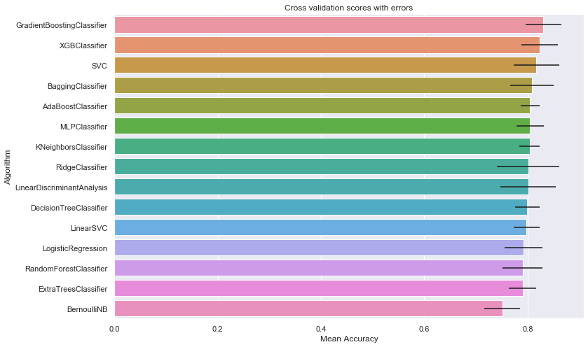
# Display the results as a bar plot
sns.barplot(cv_res_df['CrossValMeans'],
                cv_res_df['Algorithm'],
                **{'xerr':cv_std_list}
               )
plt.xlabel("Mean Accuracy")
plt.title("Cross validation scores with errors")
Text(0.5, 1.0, 'Cross validation scores with errors')
9.2. Classifiers Parameters Refinement
best_estimators = []
def gridsearch(clf, X_train, y_train, param_grid, random_state=1986, suffix='_best', scoring='accuracy',
               n_jobs=4, kfold=StratifiedKFold(n_splits=10), verbose=1, other_args={}, print_best=1):

    estimator = clf(random_state=random_state, **other_args)

    gs = GridSearchCV(estimator,
                            param_grid=param_grid,
                            cv=kfold,
                            scoring="accuracy",
                            n_jobs=n_jobs,
                            verbose=verbose)

    gs.fit(X_train,y_train)

    name_of_best_estimator=clf.__name__+suffix
    best_estimators.append((name_of_best_estimator, gs.best_estimator_))
    if print_best==1:
        print(gs.best_estimator_)

    print('Best {} score: {}%.'.format(clf.__name__, round(100*gs.best_score_,2)))
gridsearch(XGBClassifier, X_train, y_train,
           param_grid= {
#                'nthread':[4], #when use hyperthread, xgboost may become slower
#               'objective':['binary:logistic'],
#               "learning_rate": [0.01, 0.025, 0.05, 0.075, 0.1, 0.15, 0.2],
              'max_depth': [3,5,6,7],
#               'min_child_weight': [11],
#               'silent': [1],
#               'subsample': [0.8],
#               'colsample_bytree': [0.7],
              'n_estimators': [100,120], #number of trees, change it to 1000 for better results
#               'missing':[-999],
#               'seed': [1337]
           }
          )
Fitting 10 folds for each of 8 candidates, totalling 80 fits


[Parallel(n_jobs=4)]: Using backend LokyBackend with 4 concurrent workers.
[Parallel(n_jobs=4)]: Done  42 tasks      | elapsed:    3.0s


XGBClassifier(base_score=0.5, booster='gbtree', colsample_bylevel=1,
              colsample_bynode=1, colsample_bytree=1, gamma=0,
              learning_rate=0.1, max_delta_step=0, max_depth=6,
              min_child_weight=1, missing=None, n_estimators=100, n_jobs=1,
              nthread=None, objective='binary:logistic', random_state=1986,
              reg_alpha=0, reg_lambda=1, scale_pos_weight=1, seed=None,
              silent=None, subsample=1, verbosity=1)
Best XGBClassifier score: 84.07%.


[Parallel(n_jobs=4)]: Done  80 out of  80 | elapsed:    4.4s finished
gridsearch(GradientBoostingClassifier, X_train, y_train,
           param_grid= {
#     "loss":["deviance"],
    "learning_rate": [0.01, 0.025, 0.05, 0.075, 0.1, 0.15, 0.2],
#     "min_samples_split": np.linspace(0.1, 0.5, 4),
#     "min_samples_leaf": np.linspace(0.1, 0.5, 4),
#     "max_depth":[3,5,8],
#     "max_features":["log2","sqrt"],
#     "criterion": ["friedman_mse",  "mae"],
    "subsample":[0.5, 0.618, 0.8, 0.83, 0.85, 0.87, 0.9, 0.95, 1.0],
#     "n_estimators":[10]
    })
[Parallel(n_jobs=4)]: Using backend LokyBackend with 4 concurrent workers.


Fitting 10 folds for each of 63 candidates, totalling 630 fits


[Parallel(n_jobs=4)]: Done  42 tasks      | elapsed:    1.8s
[Parallel(n_jobs=4)]: Done 192 tasks      | elapsed:    7.6s
[Parallel(n_jobs=4)]: Done 442 tasks      | elapsed:   17.0s


GradientBoostingClassifier(ccp_alpha=0.0, criterion='friedman_mse', init=None,
                           learning_rate=0.15, loss='deviance', max_depth=3,
                           max_features=None, max_leaf_nodes=None,
                           min_impurity_decrease=0.0, min_impurity_split=None,
                           min_samples_leaf=1, min_samples_split=2,
                           min_weight_fraction_leaf=0.0, n_estimators=100,
                           n_iter_no_change=None, presort='deprecated',
                           random_state=1986, subsample=0.9, tol=0.0001,
                           validation_fraction=0.1, verbose=0,
                           warm_start=False)
Best GradientBoostingClassifier score: 84.29%.


[Parallel(n_jobs=4)]: Done 630 out of 630 | elapsed:   24.0s finished
gridsearch(ExtraTreesClassifier, X_train, y_train,
           param_grid={"max_depth": [None],
              "max_features": [1, 3, 10],
              "min_samples_split": [2, 3, 10],
              "min_samples_leaf": [1, 3, 10],
              "bootstrap": [False],
              "n_estimators" :[100,300],
              "criterion": ["gini"]})
[Parallel(n_jobs=4)]: Using backend LokyBackend with 4 concurrent workers.


Fitting 10 folds for each of 54 candidates, totalling 540 fits


[Parallel(n_jobs=4)]: Done  42 tasks      | elapsed:    3.9s
[Parallel(n_jobs=4)]: Done 192 tasks      | elapsed:   16.1s
[Parallel(n_jobs=4)]: Done 488 tasks      | elapsed:   35.2s
[Parallel(n_jobs=4)]: Done 540 out of 540 | elapsed:   37.1s finished


ExtraTreesClassifier(bootstrap=False, ccp_alpha=0.0, class_weight=None,
                     criterion='gini', max_depth=None, max_features=3,
                     max_leaf_nodes=None, max_samples=None,
                     min_impurity_decrease=0.0, min_impurity_split=None,
                     min_samples_leaf=3, min_samples_split=10,
                     min_weight_fraction_leaf=0.0, n_estimators=300,
                     n_jobs=None, oob_score=False, random_state=1986, verbose=0,
                     warm_start=False)
Best ExtraTreesClassifier score: 81.04%.
gridsearch(SVC, X_train, y_train,
           param_grid={'kernel': ['rbf'],
                  'gamma': [0.0005, 0.0008, 0.001, 0.005, 0.01],
                  'C': [1, 10, 50, 100, 150, 200, 250]},
          other_args={"probability": True})
Fitting 10 folds for each of 35 candidates, totalling 350 fits


[Parallel(n_jobs=4)]: Using backend LokyBackend with 4 concurrent workers.
[Parallel(n_jobs=4)]: Done  76 tasks      | elapsed:    1.9s
[Parallel(n_jobs=4)]: Done 343 out of 350 | elapsed:   11.7s remaining:    0.1s


SVC(C=100, break_ties=False, cache_size=200, class_weight=None, coef0=0.0,
    decision_function_shape='ovr', degree=3, gamma=0.005, kernel='rbf',
    max_iter=-1, probability=True, random_state=1986, shrinking=True, tol=0.001,
    verbose=False)
Best SVC score: 82.15%.


[Parallel(n_jobs=4)]: Done 350 out of 350 | elapsed:   12.2s finished
gridsearch(RandomForestClassifier, X_train, y_train,
           param_grid={"max_depth": [None],
                  "max_features": [1, 3, 10],
                  "min_samples_split": [2, 3, 10],
                  "min_samples_leaf": [1, 3, 10],
                  "bootstrap": [False],
                  "n_estimators" :[100,300],
                  "criterion": ["gini"]}
          )
Fitting 10 folds for each of 54 candidates, totalling 540 fits


[Parallel(n_jobs=4)]: Using backend LokyBackend with 4 concurrent workers.
[Parallel(n_jobs=4)]: Done  42 tasks      | elapsed:    4.6s
[Parallel(n_jobs=4)]: Done 192 tasks      | elapsed:   18.3s
[Parallel(n_jobs=4)]: Done 488 tasks      | elapsed:   38.9s


RandomForestClassifier(bootstrap=False, ccp_alpha=0.0, class_weight=None,
                       criterion='gini', max_depth=None, max_features=3,
                       max_leaf_nodes=None, max_samples=None,
                       min_impurity_decrease=0.0, min_impurity_split=None,
                       min_samples_leaf=3, min_samples_split=10,
                       min_weight_fraction_leaf=0.0, n_estimators=100,
                       n_jobs=None, oob_score=False, random_state=1986,
                       verbose=0, warm_start=False)
Best RandomForestClassifier score: 82.27%.


[Parallel(n_jobs=4)]: Done 540 out of 540 | elapsed:   40.7s finished
gridsearch(LogisticRegression, X_train, y_train,
           param_grid={"C":np.logspace(-3,3,10), "penalty":["l1","l2"]},
           other_args={'max_iter':500}
          )
[Parallel(n_jobs=4)]: Using backend LokyBackend with 4 concurrent workers.


Fitting 10 folds for each of 20 candidates, totalling 200 fits
LogisticRegression(C=0.1, class_weight=None, dual=False, fit_intercept=True,
                   intercept_scaling=1, l1_ratio=None, max_iter=500,
                   multi_class='auto', n_jobs=None, penalty='l2',
                   random_state=1986, solver='lbfgs', tol=0.0001, verbose=0,
                   warm_start=False)
Best LogisticRegression score: 79.69%.


[Parallel(n_jobs=4)]: Done 160 tasks      | elapsed:    0.5s
[Parallel(n_jobs=4)]: Done 200 out of 200 | elapsed:    0.6s finished
LDA = LinearDiscriminantAnalysis()

LDA.fit(X_train,y_train)

LDA_best = LDA

best_estimators.append(("LinearDiscriminantAnalysis_best", LDA_best))
9.3. Ensembling Final Prediction
best_estimators
[('XGBClassifier_best',
  XGBClassifier(base_score=0.5, booster='gbtree', colsample_bylevel=1,
                colsample_bynode=1, colsample_bytree=1, gamma=0,
                learning_rate=0.1, max_delta_step=0, max_depth=6,
                min_child_weight=1, missing=None, n_estimators=100, n_jobs=1,
                nthread=None, objective='binary:logistic', random_state=1986,
                reg_alpha=0, reg_lambda=1, scale_pos_weight=1, seed=None,
                silent=None, subsample=1, verbosity=1)),
 ('GradientBoostingClassifier_best',
  GradientBoostingClassifier(ccp_alpha=0.0, criterion='friedman_mse', init=None,
                             learning_rate=0.15, loss='deviance', max_depth=3,
                             max_features=None, max_leaf_nodes=None,
                             min_impurity_decrease=0.0, min_impurity_split=None,
                             min_samples_leaf=1, min_samples_split=2,
                             min_weight_fraction_leaf=0.0, n_estimators=100,
                             n_iter_no_change=None, presort='deprecated',
                             random_state=1986, subsample=0.9, tol=0.0001,
                             validation_fraction=0.1, verbose=0,
                             warm_start=False)),
 ('ExtraTreesClassifier_best',
  ExtraTreesClassifier(bootstrap=False, ccp_alpha=0.0, class_weight=None,
                       criterion='gini', max_depth=None, max_features=3,
                       max_leaf_nodes=None, max_samples=None,
                       min_impurity_decrease=0.0, min_impurity_split=None,
                       min_samples_leaf=3, min_samples_split=10,
                       min_weight_fraction_leaf=0.0, n_estimators=300,
                       n_jobs=None, oob_score=False, random_state=1986, verbose=0,
                       warm_start=False)),
 ('SVC_best',
  SVC(C=100, break_ties=False, cache_size=200, class_weight=None, coef0=0.0,
      decision_function_shape='ovr', degree=3, gamma=0.005, kernel='rbf',
      max_iter=-1, probability=True, random_state=1986, shrinking=True, tol=0.001,
      verbose=False)),
 ('RandomForestClassifier_best',
  RandomForestClassifier(bootstrap=False, ccp_alpha=0.0, class_weight=None,
                         criterion='gini', max_depth=None, max_features=3,
                         max_leaf_nodes=None, max_samples=None,
                         min_impurity_decrease=0.0, min_impurity_split=None,
                         min_samples_leaf=3, min_samples_split=10,
                         min_weight_fraction_leaf=0.0, n_estimators=100,
                         n_jobs=None, oob_score=False, random_state=1986,
                         verbose=0, warm_start=False)),
 ('LogisticRegression_best',
  LogisticRegression(C=0.1, class_weight=None, dual=False, fit_intercept=True,
                     intercept_scaling=1, l1_ratio=None, max_iter=500,
                     multi_class='auto', n_jobs=None, penalty='l2',
                     random_state=1986, solver='lbfgs', tol=0.0001, verbose=0,
                     warm_start=False)),
 ('LinearDiscriminantAnalysis_best',
  LinearDiscriminantAnalysis(n_components=None, priors=None, shrinkage=None,
                             solver='svd', store_covariance=False, tol=0.0001))]
votingC = VotingClassifier(estimators=best_estimators,
                           voting='soft', n_jobs=n_jobs)

votingC = votingC.fit(X_train, y_train)
10. Submission to Kaggle
Final predictions on the Kaggle test set:
Y_test_final_pred = votingC.predict(X_test).astype(int)
Creating a submission file:
submit_df = pd.DataFrame({ 'PassengerId': test0['PassengerId'],'Survived': Y_test_final_pred})
submit_df.to_csv("voting_submission_df.csv", index=False)
11. Results
The Kaggle website returned an accuracy score of 0.80861 (80.9%), which is in the top 6% of submissions.